# Activity levels.
mu_l = 5    # Mean of low activity levels.
mu_h = 25   # Mean of high activity levels.
mu_s = 0    # Mean of sleep activity levels.

# Activity uncertainty.
sigma_l = 7.5   # Std of low activity levels.
sigma_h = 30    # Std of high activity levels.
sigma_s = 2     # Std of activity during sleep.
sigma_t = 1.5   # Std of sleep onset/offset timing.

# The person's activity level from 0 to 1.
active_level = 0.5

# Number of days and samples of interest.
num_days = 12
num_samples = 60*24*num_daysSynthetic Data
Generating Activity from Light Schedules
This function generates an ‘activity’ schedule from an input LightSchedule.
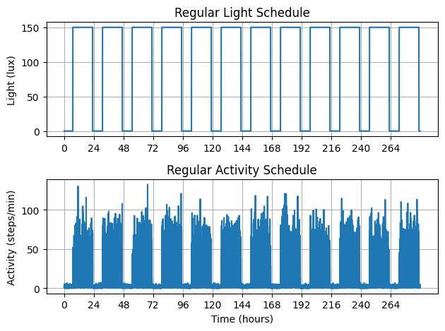
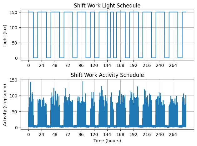
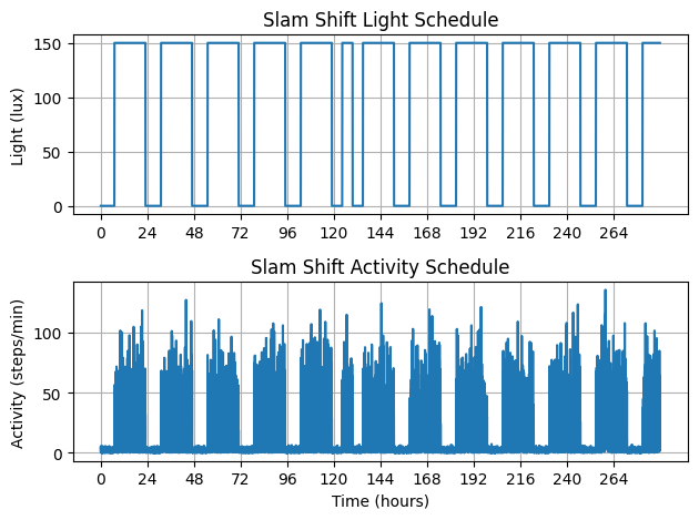
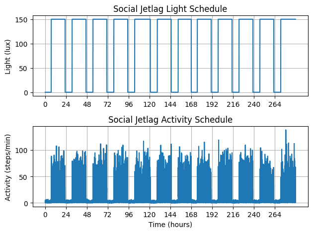
It essentially corrupts the light pulse train based on three normal distributions. When the light pulse is on, the function draws from a high or low activity distribution based on a parameter representing how active the person is, and when it is off, the function draws from a sleep activity distribution.
There are 7 parameters for the method: * mu_l - mean low activity level * mu_h - mean high activity level * mu_s - mean sleep activity level * sigma_l - std of high activity level * sigma_h - std of high activity level * sigma_s - std of sleep activity - how active the person is in their sleep * active_level - [0, 1] value representing how active the person is. When close to 1, they have a higher probability of being in the high activity distribution at any point in time
Examples
This section uses the Circadian package to generate the 4 light schedules: * Regular * Shift Work * Slam Shift * Social Jetlag
then passes each to the function to generate ‘activity’ schedules from them.
# Create the time, light and activity signals.

# Time vector.
time = np.arange(0, 24*num_days, 1/60)

# Light schedules.
regular_light = LightSchedule.Regular()
shift_light = LightSchedule.ShiftWork()
slam_light = LightSchedule.SlamShift()
social_jetlag = LightSchedule.SocialJetlag()

# Create the activity signals.
regular_activity = generate_activity_from_light(
    time, regular_light,
    mu_l, mu_h, mu_s, sigma_l, sigma_h, sigma_s,
    active_level,
)
shift_activity = generate_activity_from_light(
    time, shift_light,
    mu_l, mu_h, mu_s, sigma_l, sigma_h, sigma_s,
    active_level,
)
slam_activity = generate_activity_from_light(
    time, slam_light,
    mu_l, mu_h, mu_s, sigma_l, sigma_h, sigma_s,
    active_level,
)
social_jetlag_activity = generate_activity_from_light(
    time, social_jetlag,
    mu_l, mu_h, mu_s, sigma_l, sigma_h, sigma_s,
    active_level
)
Visualization
Here, we visualize the ‘activity’ schedules with their corresponding input light schedules.
nrows, ncols = 2, 1# Regular plots.
fig, ax = plt.subplots(nrows=nrows, ncols=ncols)
regular_light.plot(
plot_start_time=0.0,
plot_end_time=24*num_days,
num_samples=num_samples,
ax=ax[0]
)
ax[0].set_ylabel("Light (lux)")
ax[0].set_title("Regular Light Schedule")
ax[0].set_xticks(np.arange(min(time), max(time), 24))
ax[0].grid()
ax[1].plot(
time, regular_activity
)
ax[1].set_ylabel("Activity (steps/min)")
ax[1].set_xlabel("Time (hours)")
ax[1].set_title("Regular Activity Schedule")
ax[1].set_xticks(np.arange(min(time), max(time), 24))
ax[1].grid()
plt.tight_layout()
# Shift Work plots.
fig, ax = plt.subplots(nrows=nrows, ncols=ncols)
shift_light.plot(
    plot_start_time=0.0,
    plot_end_time=24*num_days,
    num_samples=num_samples,
    ax=ax[0]
)
ax[0].set_ylabel("Light (lux)")
ax[0].set_title("Shift Work Light Schedule")
ax[0].set_xticks(np.arange(min(time), max(time), 24))
ax[0].grid()
ax[1].plot(
    time, shift_activity
)
ax[1].set_ylabel("Activity (steps/min)")
ax[1].set_xlabel("Time (hours)")
ax[1].set_title("Shift Work Activity Schedule")
ax[1].set_xticks(np.arange(min(time), max(time), 24))
ax[1].grid()

plt.tight_layout()
# Slam Shift plots.
fig, ax = plt.subplots(nrows=nrows, ncols=ncols)
slam_light.plot(
    plot_start_time=0.0,
    plot_end_time=24*num_days,
    num_samples=num_samples,
    ax=ax[0]
)
ax[0].set_ylabel("Light (lux)")
ax[0].set_title("Slam Shift Light Schedule")
ax[0].set_xticks(np.arange(min(time), max(time), 24))
ax[0].grid()
ax[1].plot(
    time, slam_activity
)
ax[1].set_ylabel("Activity (steps/min)")
ax[1].set_xlabel("Time (hours)")
ax[1].set_title("Slam Shift Activity Schedule")
ax[1].set_xticks(np.arange(min(time), max(time), 24))
ax[1].grid()

plt.tight_layout()
# Social Jetlag plots.
fig, ax = plt.subplots(nrows=nrows, ncols=ncols)
social_jetlag.plot(
    plot_start_time=0.0,
    plot_end_time=24*num_days,
    num_samples=num_samples,
    ax=ax[0]
)
ax[0].set_ylabel("Light (lux)")
ax[0].set_title("Social Jetlag Light Schedule")
ax[0].set_xticks(np.arange(min(time), max(time), 24))
ax[0].grid()
ax[1].plot(
    time, social_jetlag_activity
)
ax[1].set_ylabel("Activity (steps/min)")
ax[1].set_xlabel("Time (hours)")
ax[1].set_title("Social Jetlag Activity Schedule")
ax[1].set_xticks(np.arange(min(time), max(time), 24))
ax[1].grid()

plt.tight_layout()
API Documentation
generate_activity_from_light
 generate_activity_from_light (time:numpy.ndarray,
                               light:circadian.lights.LightSchedule,
                               mu_l:float=5.0, mu_h:float=25.0,
                               mu_s:float=0.0, sigma_l:float=7.5,
                               sigma_h:float=30.0, sigma_s:float=2.0,
                               active_level:float=0.5)
Generates an ‘activity’ schedule from an input light schedule. The activity schedule produced is a corrupted version of the light schedule.
| Type | Default | Details | |
|---|---|---|---|
| time | ndarray | time points. | |
| light | LightSchedule | light schedule. | |
| mu_l | float | 5.0 | mean of low activity levels. |
| mu_h | float | 25.0 | mean of high activity levels. |
| mu_s | float | 0.0 | mean of sleep activity levels. |
| sigma_l | float | 7.5 | std of low activity levels. |
| sigma_h | float | 30.0 | std of high activity levels. |
| sigma_s | float | 2.0 | std of activity during sleep. |
| active_level | float | 0.5 | person’s activity level from 0 to 1. Represents the probability of choosing from the high or low activity distributions at any point in time. Values close to 1 increase the proportion of high activity values. |
| Returns | ndarray |