Plots

Defines functions for typical plots used in circadian science.

Actogram

slam_shift = LightSchedule.SlamShift() 
time = np.arange(0, 20*24.0, 0.10)
light_values = slam_shift(time) 

act = Actogram(time, light_vals=light_values, smooth=False)

spm = Hannay19()
trajectory = spm(time, np.array([1.0, np.pi, 0.0]), light_values)
dlmo = spm.dlmos()

act.plot_phasemarker(dlmo, color='blue')
plt.show()

MAE

dlmo_experimental = np.linspace(-12, 12., 30) 
dlmo_predicted = dlmo_experimental + np.random.normal(0, 2, len(dlmo_experimental))

plot_mae(dlmo_experimental, dlmo_predicted)
The MAE is: 4.893222072754772
Within one hour 7/30
[-3.47328784e+00  2.29203680e+01  2.14370972e+01  2.05151476e+01
 -8.28809784e-01  3.29152432e+00 -1.03521731e+00 -1.21786907e+00
  6.01046181e-01 -8.64421152e-01  2.32069554e+00 -1.20140297e+00
  1.11533503e+00 -1.35758354e+00 -1.13861312e+00  1.62675565e+00
  1.03264169e+00  1.65883693e+00  1.66964836e+00 -2.41250659e+00
  3.98410068e-01  2.24680534e+00  4.61070620e-01 -1.11127185e-02
  8.78906427e-02  1.18376113e+00  1.25223210e+00 -2.07873084e+01
 -2.31041479e+01 -5.54511532e+00]

Torus

phi1 = 12.0 + 5.0*np.random.randn(100) 
phi2 = phi1 + 5.0*np.random.randn(100)

plot_torus(phi1, phi2, scaled_by=24.0, color='darkgreen')
plt.title("Example torus plot")
plt.xlabel("$\phi_1$") 
plt.ylabel("$\phi_2$");

Stroboscopic

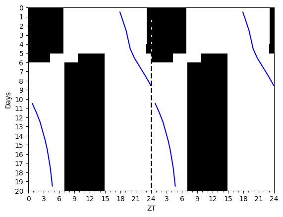
slam_shift = LightSchedule.SlamShift(shift=12.0, lux=500.0, before_days=2) 
time = np.arange(0.0, 15*24.0, 0.10)
light_values = slam_shift(time)
# Run this for a range of period parameters 
batch_dim = 50
hmodel = Hannay19({'tau': np.linspace(23.5, 24.5, batch_dim)}) 

initial_state = np.array([1.0, np.pi, 0.0]) + np.zeros((batch_dim, 3))
initial_state = initial_state.T
trajectory = hmodel(time, initial_state, light_values)

ax = plt.gca()
cmap = plt.get_cmap('jet')
for idx in range(trajectory.batch_size):
    Stroboscopic(ax, 
                 time, 
                 trajectory.states[:, 0, idx], 
                 trajectory.states[:, 1, idx], 
                 period=24.0, 
                 lw=0.50,
                 color=cmap(idx/batch_dim));
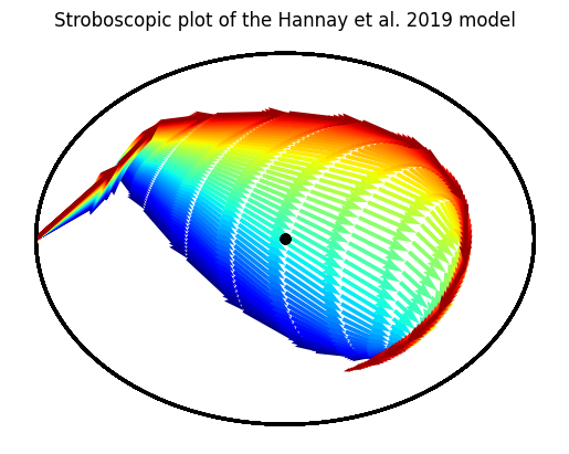
plt.title("Stroboscopic plot of the Hannay et al. 2019 model");